Lab 5: LiDAR remote sensing

Goals and Background

The goal for this lab is to gain basic knowledge on LiDAR data structure and processing. The data will be used is LiDAR point clouds int eh LAS file format. Objectives include:

1. Processing and retrieval of various surface and terrain models.
2. Processing and creation of intensity image and other derivative products from point cloud.

Recently, LiDAR is becoming more known due to the expanding areas in remote sensing. Now, there is new job creation and a significant growth in remote sensing fields.

Methods 

By first importing the .las friles into Erdas Imagine, a visual understanding is created of the points collected from the flight (Figure 1).

Figure 1. A display of each individual LAS file of the lidar point clouds. 

In ArcMap, a new LAS Dataset is created and the .las files are added to the new dataset. In the LAS Dataset Properties, statistics can be calculated pertaining to the values of all of the LAS files that were compiled (Figure 2).

Figure 2. The individual statistics provide additional information not reported under the Statistics tab for the entire LAS dataset. The minimum Z value is 517.85 and the maximum value is 1845.01.

The coordinate system for the new LAS dataset was also changed. The horizontal coordinate system (X,Y) is NAD 1983 HARN WISCRS EauClaire County (Feet) and the vertical coordinate system (Z) was adjusted to North American Vertical Datum 1988 (Meters).

Next the LAS dataset is added to ArcMap and the classification is changed to 8 classes. There is multiple ways using the LAS Dataset toolbar to examine different surface data. There are four different methods/conversion tools: elevation, aspect, slope, and contour. For this analysis, the elevation tool was used. Figure 3 shows the change in elevation with points. Figure 4 uses a interpolated elevation, where the points become shapes.

Figure 3. Point Elevation using lidar point cloud data.

Figure 4. Interpolated Elevation using lidar point cloud data. 

The high elevation points that are within Half Moon Lake are not supposed to be there. This is due to the fact that there is no defined breaklines when inputting the data. Therefore, the water that is supposed to be flat was affected by the returns during flight. 

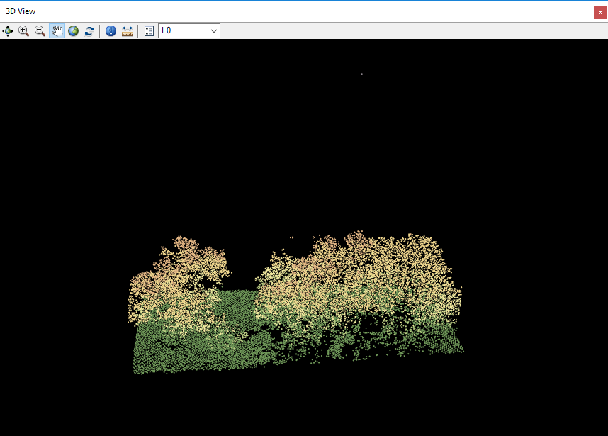
The Profile View and the 3D View are two features in the LAS Dataset Toolbar used to examine the first returns of the elevation point cloud image. One section was zoomed into that was vegetated (Figure 5). The low areas are expressed in the green color, as the points go up in elevation this could the shrubbery and then the trees in the highest elevation. There is one point that is an anomaly of a high elevation value. These points can be effected from something as simple as birds or a missed return during flight.

Figure 5. 3D View within ArcMap of lidar point cloud data.

Lidar has the capability to derive 3D images from the data. In this lab, a digital surface model (DSM) and a digital terrain model (DTM) will be created. The DSM is produced with the first return points at a spectral resolution of 2 meters. Then a hillshade will be created from the DTM and DSM. 

The parameters need to first be set in ArcMap.  The layer is set to display the points by elevation and only utilized the first returns.  Using LAS Dataset to Raster tool in ArcMap the specifications are set as follows: Value Field = Elevation, Cell Type = Maximum, Void Filling = Natural Neighbors, Cell Size =  6.56168 (approximately 2 meters). Figure 6 shows a 3D model of the earth's surface. This includes showing the elevation changes in the buildings as well as trees and other objects.

The parameters for the DTM LAS Dataset to Raster tool include: Interpolation = Binning; Cell Assignment Type = Minimum; Void Fill method = Natural_Neighbor; Sampling Type = CellSize; Sampling Value is same as that set for the DSM above. Figure 7 shows only the bare earth. This is easier to analyze the terrain when trying to see the elevation change of only the ground.

Figure 6. DSM with hillshade applied.

Figure 7. DTM with hillshade applied.

The final objective generates a lidar intensity image.The LAS Dataset is set to Points and filtered to First Return. The intensity is always captured by the first return echoes. Value Field should be set to
INTENSITY, Binning Cell Assignment Type =Average, Void fill = Natural_Neighbor, Cell Size is the same used for the DTM and DSM derived products above.

Results 

The differences between the two hillshades can be seen using the Effects Toolbar. The swipe function puts the two images side by side and the tools allows for on image to swipe over the top to see variances in the images (Figure 8).

Figure 8. Deriving DSM and DTM products from point clouds

The intensity image is dark when displayed in ArcMap. To see the true intensity of the image, the image is viewed in Erdas Imagine (Figure 9).

Figure 9. Deriving Lidar Intensity image from point cloud

Sources 

Lidar point cloud and Tile Index are from Eau Claire County, 2013.
Eau Claire County Shapefile is from Mastering ArcGIS 6th Edition data by Margaret Price, 2014.