Lab 8: Spectral signature analysis & resource monitoring

Goals and Background 

The goal of this lab is to gain experience on the measurement and interpretation of spectral signatures. This lab consists of collecting spectral signatures from remotely senses images. They will be graphed and there will be an analysis on them to verify whether they pass the spectral separability test. Also, health of vegetation and soils will be monitored using simple band ratio techniques.

Methods

Part 1: Spectral signature analysis

The satellite image was provided from the year 2000 of the Eau Claire and Chippewa Falls area in Wisconsin. 12 materials and surfaces from the image will be measured and plotted for the spectral reflectance.

1. Standing Water
2. Moving water
3. Deciduous forest
4. Evergreen forest
5. Riparian vegetation
6. Crops
7. Dry soil (uncultivated)
8. Moist soil (uncultivated)
9. Rock
10. Asphalt highway
11. Airport runway
12. Concrete surface

To obtain the spectral signatures in Erdas, the Polygon tool is utilized under the Drawing tab (Figure 1). After drawing an outline of the area of interest (AOI) to collect the spectral signature from, Signature Editor opened from the Supervised menu in the Raster tab of Erdas.  With the Signature Editor open, the Create New Signature is used from AOI and Display Mean Plot Window to add the signature from the polygon to the window and display the graph of the spectral signature.

Figure 1. Spectral images being identified using the drawing tool in Erdas. 

In the Signature Editor, Signature Name (label) was changed for each of the spectral signatures. Analyzing the spectral signatures is same time in the editor window and then selecting Multiple Signature Mode on the plot window allows you to view more than one signature (Figure 2).

Figure 2. Identified images with multiple signatures plotted on the graph. 

Part 2: Resource Monitoring

Section 1: Vegetation health monitoring 

In this section of the lab, simple band ratio is performed by implementing the normalized
difference vegetation index (NDVI) using the satellite image was provided from the year 2000 of the Eau Claire and Chippewa Falls area.

This is completed by  Raster-Unsupervised-NDVI in Erdas. In the Indices interface, the Sensor reads ‘Landsat 7 Multispectral’ in the Indices window and NDVI is highlighted. The following formula is used in order to get vegetation presence:

5 classes were used to show the abundance of vegetation presence in Eau Claire and Chippewa counties.

• Mostly water 
• No vegetation 
• Very little vegetation 
• Moderate vegetation 
• High vegetation 

Section 2: Soil health monitoring 

In this section of the lab, simple band ratio is performed by implementing the ferrous mineral ratio using the satellite image was provided from the year 2000 of the Eau Claire and Chippewa Falls area.

This is completed by Raster-Unsupervised-Indices in Erdas. In the Indices interface, the Sensor reads ‘Landsat 7 Multispectral’ in the Indices window and under Select Function, choose FERROUS MINERALS . The following formula is used in order to get ferrous mineral ratio:

5 classes were used to show the spatial distribution of ferrous minerals in Eau Claire and Chippewa counties.

• Mostly vegetation 
• Non exposed soil 
• Low ferrous minerals 
• Moderate ferrous minerals 
• High ferrous minerals

Results

Part 1: Spectral signature analysis

Analyzing the graph of reflectance from you are able to see the variation between standing water and moving water.  The variation displayed between the two water surfaces is explained through Specular and Diffuse reflection. The movement and ripples in the moving water give it diffuse reflection which send the reflections in all directions and reduces the intensity.  Where as the standing water is smooth has a more specular reflection, which sends the reflectance back with a higher intensity.  Multiple variations of this type of analysis can be done from the spectral information gathered in this manner.

Figure 3. Signature Editor with all of the spectral images identified. 

Figure 4. Signature mean plot with all 12 images plotted. 

Part 2: Resource Monitoring

Section 1: Vegetation health monitoring 

Figure 5. Vegetation Presence in Eau Claire and Chippewa County ranked with 5 classes. 

Section 2: Soil health monitoring 

Figure 6. Distribution of Ferrous Minerals in Eau Claire and Chippewa County based on 5 classes. 

Sources

Satellite image is from Earth Resources Observation and Science Center, United States Geological Survey.  

Lab 7: Photogrammetry

Goals and Background

The goal of this lab is to obtain skills needed to perfomr key photogrammetric tasks on aerial photographs and satellite images. This lab is designed to understand  the math behind the calculations of photographic scales, measurement of areas and perimeters of features, and calculating relief displacement. There is an introduction to stereoscopy and performing orthorecticication on satellite images. 

Methods

Scales, Measurements, and Relief Displacement

The first part of this lab is calculating the scale of nearly vertical aerial photographs. Calculating the scale can be done in a couple different manners.

First, the scale was calculated measuring two points on the aerial photograph and compare that measurement to the real world distance.  Though this is a great and simple method it isn't always possible to obtain a measurement in the real world. 

Utilizing an image labeled with point A to point B, the measure with my ruler and got a measurement of 2.5 inches (Figure 1). The dimension in the real world from point A to point B was 8822.47 ft. The real world dimension to inches which was 105869.64. The expression to get the scale value is below:

2.5 in./8822.47 ft = 2.5/105869.64 = 1:42,348

Figure 1. Aerial Photo of the City of Eau Claire displaying points A to B. This image is not shown to the scale the that measurements were taken. 

Photographic scale can be calculated without a true real world measurement as long as the focal length of the camera and the flying height above the terrain of the aircraft is known.  The information given was as follows: Aircraft altitude= 20,000 ft, Focal length of camera=152 mm, and the elevation of the area in the photograph=769 ft. The photographic scale can be calculated using the formula: 

S = F/(H-h)

S =  .4986816/(20000-796)

The formula gives a scale of 1:40,000 when it is rounded to the nearest thousand. 

Measurement of areas of features on aerial photographs

For this section of the assignment I will be utilizing Erdas Imagine to calculate the area of a lagoon in an aerial image (Figure 2).

By utilizing the polygon measurement tool in the measure tool bar, the area of the lagoon provided can be calculated. This is don by tracing the outline of the lagoon. From there different measurements can be changed to get multiple measurements. The results included: 

• Area = 38.0736 ha and 94.0820 acres
• Perimeter = 8390.74 meters and 5.213767 miles

Figure 2. Photo used in Erdas to measure the area and perimeter of the lagoon located on the west side of the image.

Calculating relief displacement from object height

Relief displacement is the variation of objects and features within an aerial image from their true planimetric position on the ground.  Assessing Figure 3, the smoke stack (labeled 'A') is at an angle. Therefore, the smoke stack is showing displacement related to the location of the Principal Point and the location of the feature. 

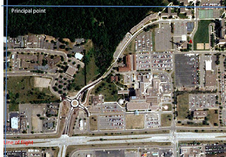
Figure 3. Aerial photo used to show relief displacement of the smoke stack at point A. This image is not shown to the scale the that measurements were taken. 

 

The scale of the image is 1:3209 and the camera height is 3,980 ft. To calculate relief displacement the formula is D= hr/H.

• h = the height of the object in the real world
• r = radial distance from the principal point to the top of the displaced object
• H = the height of the camera when the image was taken

In order to complete the formula, the real world smoke stack needed to be measured from the distance from the principal point to the top of the smoke stack.  Using the scale and a ruler the determined height of the smoke stack was 802.25 inches and the radial distance from the principal point was 5 inches. 

802.25 in. *5 in. / 3209 ft = 802.25 in * 5 in. / 38508 in. = 0.1042

To correct this image the smoke stack would have to be pushed back the .1042 inches to make vertical.

Stereoscopy

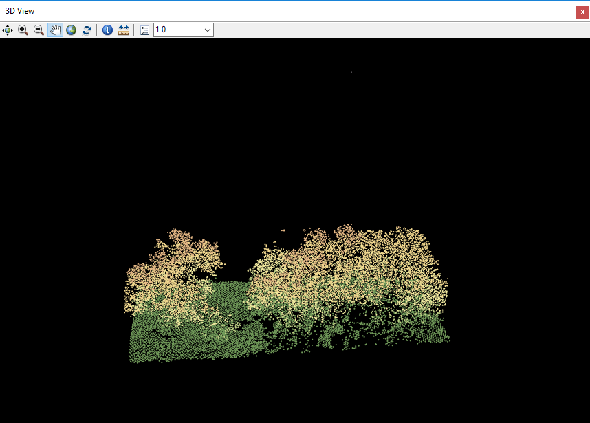
Stereoscopy is the science of depth perception utilizing your eyes or other tools to view a 2 dimensional (2D) image in 3 dimensions (3D).  The tools Stereoscope, Anaglyph and Polaroid glasses, were used to develop and view 2D images in 3D. Erdas Imagine was used to create an Anaglyph.  Anaglyph tool is selected in the Terrain menu tab.  An aerial image of the City of Eau Calire and a Digital Elevation Model (DEM) was used in the Anaglyph Generation menu.  Then  next step is to run the tool. Once this is complete, the image can be opened up in Erdas and viewed using 3D glasses to show a different way of looking at a 3D model. 

Orthorectification

Orthorectification refers to simultaneously removes positional and elevation errors from one or multiple aerial photographs or satellite images.  This process requires the analyst to obtain real world x,y, and z coordinates of pixels on aerial images and photographs.  Orthorectified images can be utilized to create many products such as DEM's, and Stereopairs.

This section uses Erdas Imagine Lecia Photogrammetric Suite (LPS).  This tool with in Erdas Imagine is used for triangulation, orthorectification with digital photogrammetry collected by varying sensors.  Additionally, it can be used to extract digital surface and elevation models. Two images were provided and placed in Erdas. Because the images overlapped they needed to be corrected. 

First, a New Block File was created in the Imagine Photogrammetry Project Manager window.  In the Model Setup dialog window the Geometric Model Category was set to Plynomial-based Pushbroom and selected SPOT Pushbroom in the second section window.  In the Block Property Setup I set the projection to UTM, the Spheroid Name to Clarke 1866, and the Datum to NAD 27 (CONUS).  

The next step the point measurement tool was activated to collect GCP's.  The point measurement tool was set to Classic Point Measurement Tool.  Using the Reset Horizontal Reference icon, the GCP Reference Source was set to Image Layer. Then, 11 GCP's were located on the uncorrected image and the reference image (Figure 4). 

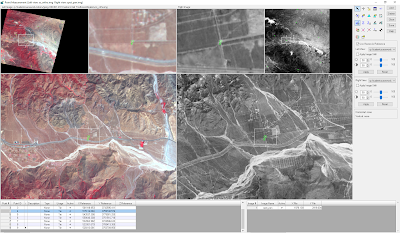
Figure 4. Screen shot of the Imagine Photogrammetry Project Manager window with the first 9 GCPs and their information.

Vertical Reference Source needed to be updated and collect elevation information utilizing a DEM.  Clicking on the Reset Vertical Reference Source icon opens a menu to set the Vertical Reference Source to a selected DEM.  After selecting the DEM in the menu all of the values in the cell array were selected and the Z Values were updated on Selected Points icon (Figure 5).  

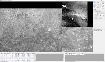
Figure 5. Updated GCP points after the Z values were added.

After all of the GCP's were added and the elevation was set to the first image, the second image needed to be imported for correction.  The Type and Usage had to be set for each of the control points.  Type to Full and the Usage to Control for each of the GCP's. The Add Frame icon and add the second image for orthorectification was used.  I set the parameters and verified the SPOT Sensor specifications the same as the first image.  Only the GCP's that were within the overlap of the two images were corrected (1,2,5,6,8,9,12).

Lastly, Automatic Tie Point Generation Properties icon to calculate tie points between the two images. Tie points are points which have an unknown ground coordinates but are able to be visually identified in the overlap area of images. The coordinates of the tie points are calculated during a process called block triangulation.  Block triangulation requires a minimum of 9 tie points to process.

In the Automatic Tie Point Generation Properties window set the Image used to All Available and the Initial Type to Exterior/Header/GCP.  Under the distribution tab the Intended Number of Points/Images were set to 40.

Triangulation tool was ran after setting the parameters as follows:

• Iterations wtih Relaxation was set to a value of 3
• Image Coordinate Units for Report was set to Pixels.
• Type to Same as Weighted Values and the X,Y, and Z values to 15 to assure the GCP's are accurate with in 15 meters. 

After running the tool a report was displayed to asses the accuracy (Figure 6). 

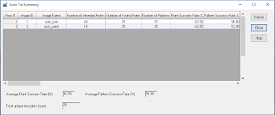
Figure 6. AutoTie Summary from Erdas Imagine.

The final step including running the Ortho Resampling Process. 

Results

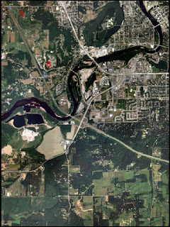
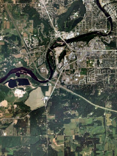
The final results of the Orthorectification resulted in accurately positioned images (Figure 7).  

Figure 7. Final product of the two images after Orthorectification.

Sources

National Agriculture Imagery Program (NAIP) images are from United States Department of Agriculture, 2005. 

Digital Elevation Model (DEM) for Eau Claire, WI is from United States Department of Agriculture Natural Resources Conservation Service, 2010. 

Lidar-derived surface model (DSM) for sections of Eau Claire and Chippewa are from Eau Claire County and Chippewa County governments respectively. 

Spot satellite images are from Erdas Imagine, 2009. 

Digital elevation model (DEM) for Palm Spring, CA is from Erdas Imagine, 2009. 

National Aerial Photography Program (NAPP) 2 meter images are from Erdas Imagine, 2009. 

Lab 6: Geometric Correction

Goals and Background 

The goal for this lab is to introduce an image preprocessing exercise called geometric correction. This will develop skills using two major types of geometric correction that are typically performed on satellite images as part of the preprocessing activities that come before the extraction of biophysical and sociocultural information from satellite images. Rectification will be used in this lab. Rectification is the process of converting a data file coordinate or grid system known as a reference system.

1. Image-to-Map Rectification: this type of geometric correction utilized a map coordinate system to rectify/transform the image pixel coordinates.
2. Image-to-Image Rectification: this type of geometric correction uses a previously corrected image of the same location to rectify/transform the image data pixel coordinates. 

Methods

Image-to-Map Rectification was the first type of geometic correction used. The USGS 7.5 minute digital raster graphic (DRG) was used to correct the Landsat TM image. Control Points will be used in ERGAS Imagine under the Multispectral tab to perform the correction. The Geometic Model is set to Polynomial and the first order polynomial equation is used. The USGS DRG is also set as the reference map. When you are using a first order polynomial, there needs to be a minimal of 3 ground control points (GCP)

To correct the image, GCP will be placed on both of the images in the same locations. Once four GCPs were placed they need to be adjusted. By looking at the Root Mean Square (RMS) error, it can determine the accuracy between the exact locations on the two images. The industry standard for remote sensing is 0.5 RMS error or below. Since this is an introductory lab, the RMS error needed to be less than 2. The points could be adjusted until the values were below the recommended values. The RMS error total for this exercise ended up being 0.1413 (Figure 1).

Figure 1. Image-to-Map Rectification: Multipoint Geometic Correction with 4 GCP and a RMS error value of 0.1413. 

For part one, even with an RMS error value of 0.1413, there was minimal error in the image that was corrected to begin with. Therefore, displaying the correction was difficult, shown in Figure 2. The final images shown below were resampled using the defaults of the display function to create the new geometrically corrected image. 

Figure 2. Corrected image next to original image with error. 

The second method was Image-to-Image Rectification. The settings for Control Points were all the same except that the equation was changed to a third order polynomial. A third order needs a minimum of 10 GCP. This lab included 12 GCP to get an RMS error total of 0.2027 (Figure 3).

Figure 3. Image-to-Image Rectification: Multipoint Geometic Correction with 12 GCP and a RMS error value of 0.2027.

When the correction was completed, the image was resampled this time using the bilinear interpolation. Using the slide function in ERDAS Imagine, the corrected image can be seen on top of the original image (Figure 4).

Figure 4. Viewer swipe with corrected image and reference image.

Results 

 This lab created a basic understanding of geometric correction. In order to have an accurate analysis, geometrically corrected images are essential. The error may not always be obvious, but when it is zoomed in a difference can be detected. Locating areas that are good for GCP takes practice. But you can never have enough GCP.

Sources

Satellite images are from Earth Resources Observation and Science Center, United States Geological Survey.
Digital raster graphic (DRG) is from Illinois Geospatial Data Clearing House.

Lab 5: LiDAR remote sensing

Goals and Background

The goal for this lab is to gain basic knowledge on LiDAR data structure and processing. The data will be used is LiDAR point clouds int eh LAS file format. Objectives include:

1. Processing and retrieval of various surface and terrain models.
2. Processing and creation of intensity image and other derivative products from point cloud.

Recently, LiDAR is becoming more known due to the expanding areas in remote sensing. Now, there is new job creation and a significant growth in remote sensing fields.

Methods 

By first importing the .las friles into Erdas Imagine, a visual understanding is created of the points collected from the flight (Figure 1).

Figure 1. A display of each individual LAS file of the lidar point clouds. 

In ArcMap, a new LAS Dataset is created and the .las files are added to the new dataset. In the LAS Dataset Properties, statistics can be calculated pertaining to the values of all of the LAS files that were compiled (Figure 2).

Figure 2. The individual statistics provide additional information not reported under the Statistics tab for the entire LAS dataset. The minimum Z value is 517.85 and the maximum value is 1845.01.

The coordinate system for the new LAS dataset was also changed. The horizontal coordinate system (X,Y) is NAD 1983 HARN WISCRS EauClaire County (Feet) and the vertical coordinate system (Z) was adjusted to North American Vertical Datum 1988 (Meters).

Next the LAS dataset is added to ArcMap and the classification is changed to 8 classes. There is multiple ways using the LAS Dataset toolbar to examine different surface data. There are four different methods/conversion tools: elevation, aspect, slope, and contour. For this analysis, the elevation tool was used. Figure 3 shows the change in elevation with points. Figure 4 uses a interpolated elevation, where the points become shapes.

Figure 3. Point Elevation using lidar point cloud data.

Figure 4. Interpolated Elevation using lidar point cloud data. 

The high elevation points that are within Half Moon Lake are not supposed to be there. This is due to the fact that there is no defined breaklines when inputting the data. Therefore, the water that is supposed to be flat was affected by the returns during flight. 

The Profile View and the 3D View are two features in the LAS Dataset Toolbar used to examine the first returns of the elevation point cloud image. One section was zoomed into that was vegetated (Figure 5). The low areas are expressed in the green color, as the points go up in elevation this could the shrubbery and then the trees in the highest elevation. There is one point that is an anomaly of a high elevation value. These points can be effected from something as simple as birds or a missed return during flight.

Figure 5. 3D View within ArcMap of lidar point cloud data.

Lidar has the capability to derive 3D images from the data. In this lab, a digital surface model (DSM) and a digital terrain model (DTM) will be created. The DSM is produced with the first return points at a spectral resolution of 2 meters. Then a hillshade will be created from the DTM and DSM. 

The parameters need to first be set in ArcMap.  The layer is set to display the points by elevation and only utilized the first returns.  Using LAS Dataset to Raster tool in ArcMap the specifications are set as follows: Value Field = Elevation, Cell Type = Maximum, Void Filling = Natural Neighbors, Cell Size =  6.56168 (approximately 2 meters). Figure 6 shows a 3D model of the earth's surface. This includes showing the elevation changes in the buildings as well as trees and other objects.

The parameters for the DTM LAS Dataset to Raster tool include: Interpolation = Binning; Cell Assignment Type = Minimum; Void Fill method = Natural_Neighbor; Sampling Type = CellSize; Sampling Value is same as that set for the DSM above. Figure 7 shows only the bare earth. This is easier to analyze the terrain when trying to see the elevation change of only the ground.

Figure 6. DSM with hillshade applied.

Figure 7. DTM with hillshade applied.

The final objective generates a lidar intensity image.The LAS Dataset is set to Points and filtered to First Return. The intensity is always captured by the first return echoes. Value Field should be set to
INTENSITY, Binning Cell Assignment Type =Average, Void fill = Natural_Neighbor, Cell Size is the same used for the DTM and DSM derived products above.

Results 

The differences between the two hillshades can be seen using the Effects Toolbar. The swipe function puts the two images side by side and the tools allows for on image to swipe over the top to see variances in the images (Figure 8).

Figure 8. Deriving DSM and DTM products from point clouds

The intensity image is dark when displayed in ArcMap. To see the true intensity of the image, the image is viewed in Erdas Imagine (Figure 9).

Figure 9. Deriving Lidar Intensity image from point cloud

Sources 

Lidar point cloud and Tile Index are from Eau Claire County, 2013.
Eau Claire County Shapefile is from Mastering ArcGIS 6th Edition data by Margaret Price, 2014. 

Lab 4: Miscellaneous Image Functions

Goal and Background

The goal of this lab was to demonstrate how to use various tools needed to analyze remote sensing imagery. These tools consist of: 

1. Delineating a study area from a  larger satellite image scene.
2. Demonstrate how spatial resolution images can be optimized for visual interpretation purposes.
3. Introduce some radiometric enhancement techniques in optical images. 
4. Linking a satellite image to Google Earth.
5. Introduce students to various methods of resampling satellite images. 
6. Begin image mosaicking.
7. Introduce binary change detection with the use of simple graphical modelling. 

At the end of this lab, a better understanding of the methods described will be obtained in order to improve interpretation. 

Methods

All of the objectives in this lab were completed using ERDAS Imagine 2016.

Subsetting/Area of Interest (AOI)

Often when you are assessing satellite images, the image will be larger then your area of interest (AOI). There are two ways to subset satellite images. The first ways is to create a rectangle or box in the image scene by using the Inquire box. This eliminates the surrounding unnecessary imagery and only projects the AOI.
When the AOI is an irregular shape, the second options is delineate an AOI  using a shapefile of that specified area. First, the Shapefile of Eau Claire and Chippewa County was imported into ERDAS over the satellite imagery. After the shapefile was saved as an AOI layer, the raster subset & clip tool eliminates the rest of the data to only show the AOI.

Image Fusion and Image Optimization 

A higher spatial resolution can be created from a coarse resolution by using pansharpen. Pansharpening takes the panchromatic band, which has a high resolution, and merges it with the reflective band of lower resolution.
Merge Resolution was used in the Pan Sharpen function to create the multispectral image. The method was multiplicative and the resampling technique used in this section was the Nearest Neighbor. Once this is completed the 15 meter panchromatic image is merged with the 30 meter reflective image.

Radiometric Enhancement Techniques

The radiometric enhancement techniques used in this section are preliminary. One use reducing the amount of haze in a satellite image. This is completed by choosing Radiometric in the raster tab and searching for Haze Reduction. 

Linking a satellite image to Google Earth

The option to link a satellite image to Google Earth was a recent development in ERDAS 2011. This tool is useful for image classification, as Google Earth from GeoEye high resolution satellite are most recent. Once the image is connected to Google Earth, the views can be synced together. This is known as the selective image interpolation key. 

Resampling Satellite Images

The purpose of resampling is to change the size of pixels. Resampling can increase (resample up) or decrease (resample down) the size of pixels to meet the analytical needs. Under the spatial functions, the Resample Pixel Size is selected. There is three different resampling methods: Nearest Neighebor, Bilinear Interpolation, and Cubic Convolution. This section uses the Nearest Neighbor and Bilinear Interpolation. The images were then placed side by size to compare the pixel sizes between the two methods. 

Image Mosaicking

Image mosaicking is used when two satellite images are needed in order to create the area of interest. ERDAS has multiple options to mosaic images. The two in this section that will be explored are Moasic Express and Mosaic Pro. First, the two images are brought in and making sure the Multiple options are set to Multiple Images in Virtual Mosaic and the Raster Options have Background Transparent checked. 

Mosaic Express is the easy and brief method to combine images for basic visual interpretation. This method should not be used to serious image interpretation. Mosaic Express is completed by imported the previous two images with the criteria above. In the Raster tab, selected Mosaic Express under Mosaic. Input the two images and accept default model parameters.

Mosaic Pro is a function used within ERDAS Imagine. This option gives you a plethora of options to give the image the best representation by setting the correct parameters. Like previously, the two images area added into Pro. Before adding the images, the Compute Active Area needs to be selected. The Histogram Matching needs to be selected for the matching methods for the overlap areas.

Image Differencing: Binary Change Detection

The image differencing will be used to estimate the brightness values of pixels that changed in the AOI between August 1991 and August 2011. Using the Two Input Operators (making the operator (-)), the histogram from the image metadata can show the range of brightness values. The histogram was divided up into sections that showed the pixels that did not change between dates and their mean and the pixels that changed substantially between dates (Figure 1). These values are determined using the Mean + 1.5(Standard Deviation).

Figure 1. Values less than -24.1 and greater than 72.2 were areas that showed a great deal of change. 

The next step is to map out the changes that occured in Eau Claire County and the four other neighboring counties between August 1991 and August 2011. This is done by using the equation: 

ΔBVijk = BVijk(1) – BVijk(2) + c

This function can be completed using Model Maker. Figure 2 shows a sample of the first model to establish the areas of change. 

Figure 2. Equation to find the change: $n1_ec_envs_2011_b4 - $n2_ec_envs_1991_b4 + 127.

Another model will be created to show the pixels that have changed in the study area using the change/no change threshold. The conditions are as followed:

EITHER 1 IF ( $n1_ec_91> change/no change threshold value) OR 0 OTHERWISE

After the feature has been created, it can be uploaded into ArcMap. The areas that show change will clearly appear in the study area. 

Results

Subsetting/Area of Interest

Figure 3. Eau Claire and Chippewa County (AOI) that was obtained from a larger satellite image. 

Image Fusion and Image Optimization 

Figure 4. Compares the original image (left) to the pansharpened image (right) to compare the resolution. 

Radiometric Enhancement Techniques

Figure 5. Origional Image (left) compared to the Haze Reduction Image (right).

Linking a satellite image to Google Earth

Figure 6. Image from ERDAS synced to the same area on Google Earth.

Resampling Satellite Images

Figure 7. Synconized view of the Nearest Neighbor (left) and the Bilinear Interpolation (right) resampling methods to compare pixel size. 

Image Mosaicking

Mosaic Express

Figure 8. Variance in Mosaic Expressed Image.

MosaicPro

Figure 9. Smoothness in MosaicPro image.

Image Differencing: Binary Change Detection

Figure 10. the Binary Change Detection in Eau Claire County and the four other neighboring counties between August 1991 and August 2011. 

Sources

Satellite images are from Earth Resources Observation and Science Center, United States Geological Survey. 

Shapefile is from Mastering ArcGIS 6th edition Dataset by Maribeth Price, McGraw Hill. 2014.