Goal and Background
The goal of this lab was to demonstrate how to use various tools needed to analyze remote sensing imagery. These tools consist of:
- Delineating a study area from a larger satellite image scene.
- Demonstrate how spatial resolution images can be optimized for visual interpretation purposes.
- Introduce some radiometric enhancement techniques in optical images.
- Linking a satellite image to Google Earth.
- Introduce students to various methods of resampling satellite images.
- Begin image mosaicking.
- Introduce binary change detection with the use of simple graphical modelling.
At the end of this lab, a better understanding of the methods described will be obtained in order to improve interpretation.
Methods
All of the objectives in this lab were completed using ERDAS Imagine 2016.
Subsetting/Area of Interest (AOI)
Often when you are assessing satellite images, the image will be larger then your area of interest (AOI). There are two ways to subset satellite images. The first ways is to create a rectangle or box in the image scene by using the Inquire box. This eliminates the surrounding unnecessary imagery and only projects the AOI.
When the AOI is an irregular shape, the second options is delineate an AOI using a shapefile of that specified area. First, the Shapefile of Eau Claire and Chippewa County was imported into ERDAS over the satellite imagery. After the shapefile was saved as an AOI layer, the raster subset & clip tool eliminates the rest of the data to only show the AOI.
Merge Resolution was used in the Pan Sharpen function to create the multispectral image. The method was multiplicative and the resampling technique used in this section was the Nearest Neighbor. Once this is completed the 15 meter panchromatic image is merged with the 30 meter reflective image.
Image mosaicking is used when two satellite images are needed in order to create the area of interest. ERDAS has multiple options to mosaic images. The two in this section that will be explored are Moasic Express and Mosaic Pro. First, the two images are brought in and making sure the Multiple options are set to Multiple Images in Virtual Mosaic and the Raster Options have Background Transparent checked.
Mosaic Express is the easy and brief method to combine images for basic visual interpretation. This method should not be used to serious image interpretation. Mosaic Express is completed by imported the previous two images with the criteria above. In the Raster tab, selected Mosaic Express under Mosaic. Input the two images and accept default model parameters.
Mosaic Pro is a function used within ERDAS Imagine. This option gives you a plethora of options to give the image the best representation by setting the correct parameters. Like previously, the two images area added into Pro. Before adding the images, the Compute Active Area needs to be selected. The Histogram Matching needs to be selected for the matching methods for the overlap areas.
When the AOI is an irregular shape, the second options is delineate an AOI using a shapefile of that specified area. First, the Shapefile of Eau Claire and Chippewa County was imported into ERDAS over the satellite imagery. After the shapefile was saved as an AOI layer, the raster subset & clip tool eliminates the rest of the data to only show the AOI.
Image Fusion and Image Optimization
A higher spatial resolution can be created from a coarse resolution by using pansharpen. Pansharpening takes the panchromatic band, which has a high resolution, and merges it with the reflective band of lower resolution.Merge Resolution was used in the Pan Sharpen function to create the multispectral image. The method was multiplicative and the resampling technique used in this section was the Nearest Neighbor. Once this is completed the 15 meter panchromatic image is merged with the 30 meter reflective image.
Radiometric Enhancement Techniques
The radiometric enhancement techniques used in this section are preliminary. One use reducing the amount of haze in a satellite image. This is completed by choosing Radiometric in the raster tab and searching for Haze Reduction.
Linking a satellite image to Google Earth
The option to link a satellite image to Google Earth was a recent development in ERDAS 2011. This tool is useful for image classification, as Google Earth from GeoEye high resolution satellite are most recent. Once the image is connected to Google Earth, the views can be synced together. This is known as the selective image interpolation key.
Resampling Satellite Images
The purpose of resampling is to change the size of pixels. Resampling can increase (resample up) or decrease (resample down) the size of pixels to meet the analytical needs. Under the spatial functions, the Resample Pixel Size is selected. There is three different resampling methods: Nearest Neighebor, Bilinear Interpolation, and Cubic Convolution. This section uses the Nearest Neighbor and Bilinear Interpolation. The images were then placed side by size to compare the pixel sizes between the two methods.
Image Mosaicking
Image mosaicking is used when two satellite images are needed in order to create the area of interest. ERDAS has multiple options to mosaic images. The two in this section that will be explored are Moasic Express and Mosaic Pro. First, the two images are brought in and making sure the Multiple options are set to Multiple Images in Virtual Mosaic and the Raster Options have Background Transparent checked. Mosaic Express is the easy and brief method to combine images for basic visual interpretation. This method should not be used to serious image interpretation. Mosaic Express is completed by imported the previous two images with the criteria above. In the Raster tab, selected Mosaic Express under Mosaic. Input the two images and accept default model parameters.
Mosaic Pro is a function used within ERDAS Imagine. This option gives you a plethora of options to give the image the best representation by setting the correct parameters. Like previously, the two images area added into Pro. Before adding the images, the Compute Active Area needs to be selected. The Histogram Matching needs to be selected for the matching methods for the overlap areas.
Image Differencing: Binary Change Detection
The image differencing will be used to estimate the brightness values of pixels that changed in the AOI between August 1991 and August 2011. Using the Two Input Operators (making the operator (-)), the histogram from the image metadata can show the range of brightness values. The histogram was divided up into sections that showed the pixels that did not change between dates and their mean and the pixels that changed substantially between dates (Figure 1). These values are determined using the Mean + 1.5(Standard Deviation).
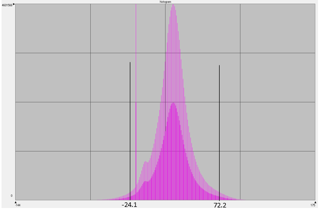 |
| Figure 1. Values less than -24.1 and greater than 72.2 were areas that showed a great deal of change. |
The next step is to map out the changes that occured in Eau Claire County and the four other neighboring counties between August 1991 and August 2011. This is done by using the equation:
ΔBVijk = BVijk(1) – BVijk(2) + c
This function can be completed using Model Maker. Figure 2 shows a sample of the first model to establish the areas of change.
 |
| Figure 2. Equation to find the change: $n1_ec_envs_2011_b4 - $n2_ec_envs_1991_b4 + 127. |
Another model will be created to show the pixels that have changed in the study area using the change/no change threshold. The conditions are as followed:
EITHER 1 IF ( $n1_ec_91> change/no change threshold value) OR 0 OTHERWISE
After the feature has been created, it can be uploaded into ArcMap. The areas that show change will clearly appear in the study area.
Results
Subsetting/Area of Interest
 |
| Figure 3. Eau Claire and Chippewa County (AOI) that was obtained from a larger satellite image. |
Image Fusion and Image Optimization
 |
| Figure 4. Compares the original image (left) to the pansharpened image (right) to compare the resolution. |
Radiometric Enhancement Techniques
 |
| Figure 5. Origional Image (left) compared to the Haze Reduction Image (right). |
Linking a satellite image to Google Earth
 |
| Figure 6. Image from ERDAS synced to the same area on Google Earth. |
Resampling Satellite Images
 |
| Figure 7. Synconized view of the Nearest Neighbor (left) and the Bilinear Interpolation (right) resampling methods to compare pixel size. |
Image Mosaicking
Mosaic Express
 |
| Figure 8. Variance in Mosaic Expressed Image. |
MosaicPro
 |
| Figure 9. Smoothness in MosaicPro image. |
Image Differencing: Binary Change Detection
 |
| Figure 10. the Binary Change Detection in Eau Claire County and the four other neighboring counties between August 1991 and August 2011. |
Sources
Satellite images are from Earth Resources Observation and Science
Center, United States Geological Survey.
Shapefile is from Mastering ArcGIS 6th edition Dataset
by Maribeth Price, McGraw Hill. 2014.


